Adjust data to your needs
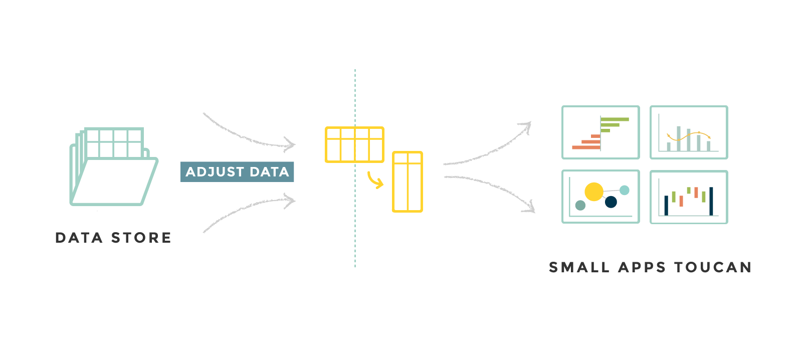
To adjust data to your charts, we have several tools to adapt the data.
The simpliest way is to simply link the good domain to your chart. You
can also use data manipulations in MongoDB or usual functions created by
Toucan Toco called postprocess.
Tutorial: Product Corporation
You can download the CSV file for our tutorial.
data-product-corporation.csv affected to the domain: data-product.
Note
You can use comments in your query to explain the differents steps you’re doing.
Simply use this syntax :
$comment: "This is a commentary to explain what I'm doing in my query"
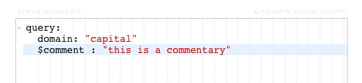
comments
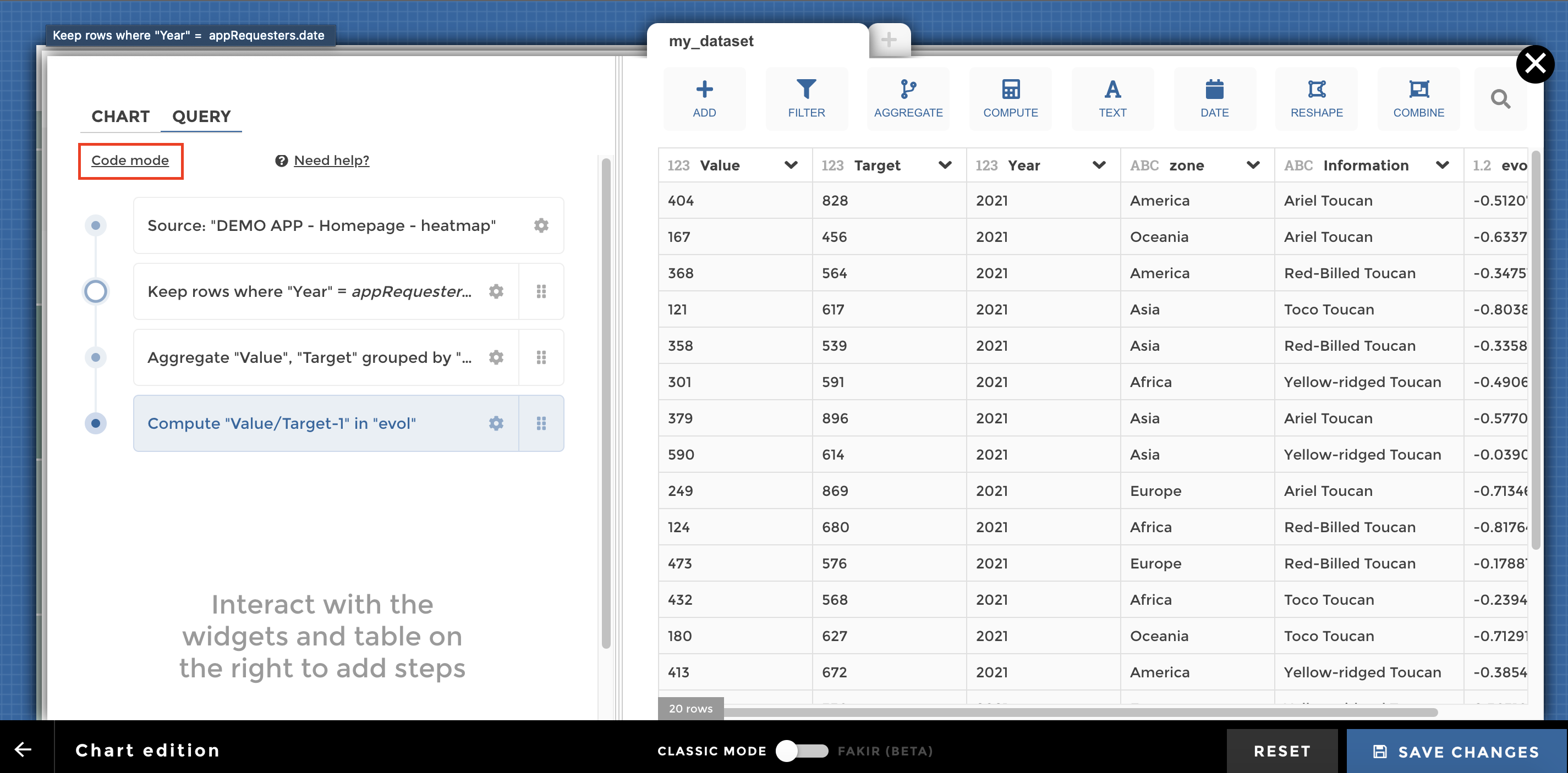
YouPrep™
YouPrep™ is a graphical tool that will let you transform your datasets without having to write the query manually by yourself.
YouPrep™ will help you with most of the data transformations you need (filtering, computation, aggregation, text and date operations, reshaping, combining several datasets)
For information, we built YouPrep™ as an open source project that can be extended by the community. Today, we translate user interactions into Mongo query language. Tomorrow, we want to be able to translate languages ranging from our custom postprocess language (see below on this page) to SQL. The project is called WeaverBird.
For a detailed documentation on how to use the user interface, please see this dedicated page.
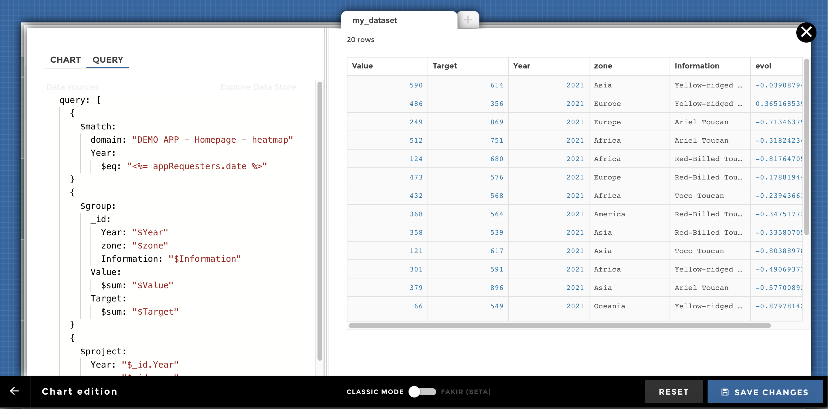
Switch to code mode
If you feel stuck on YouPrep™, you can switch to code mode for more advanced transformations:
Be careful, it is a one way journey: you cannot go back from code mode to YouPrep™ (at least not at the moment). But you will not lose what you’ve already done with YouPrep™ ! When clicking on “Switch to code mode”, you can start from the query already generated by YouPrep™:
Dynamic queries
In your data query you can use variables instead of raw values. Those variables come from the requesters that you define in your stories or on your home (for views and dates). As you select a value in a requester, the corresponding variable takes the selected value. It’s very powerful to filter your data and make your queries lighter and more dynamic.
In YouPrep™, when you are configuring a step, some fields will display the variable button at hover, indicating that you can use a variable:
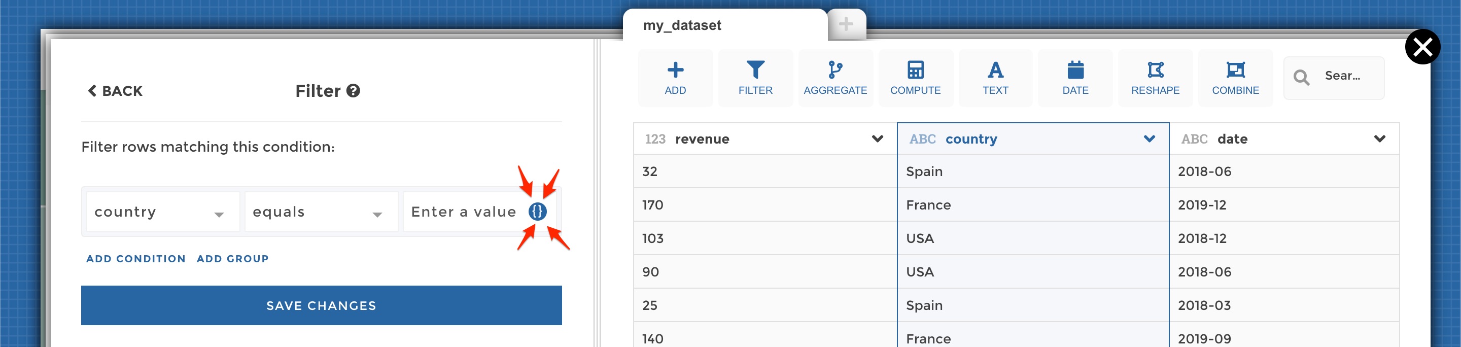
Variables button
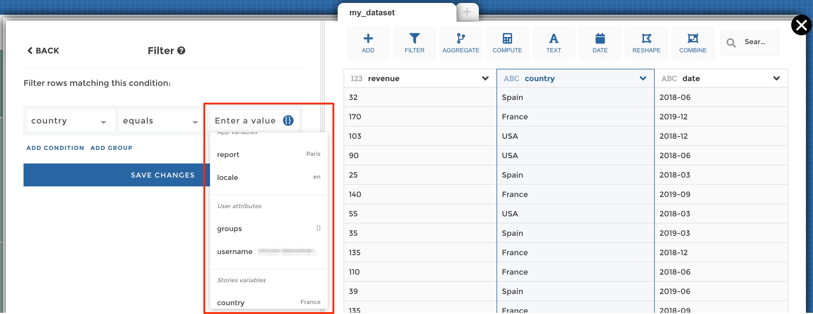
Variables dropdown
In the screenshot above, you can see the list of all available variables:
- App variables are those derived from you global app requesters, i.e. views and dates selectors (those requesters are always available in all your stories)
- User variables are those derived from the current user viewing the app. It can be useful to use those variables when you need to filter your queries based on the user’s user group, id etc.
- Story variables are those derived from the requesters that you define in a given story
Advanced variables
At the bottom of the variables drodpown you will find an “Advanced variable” button. This will allow you to define custom, more complex variables in code mode.
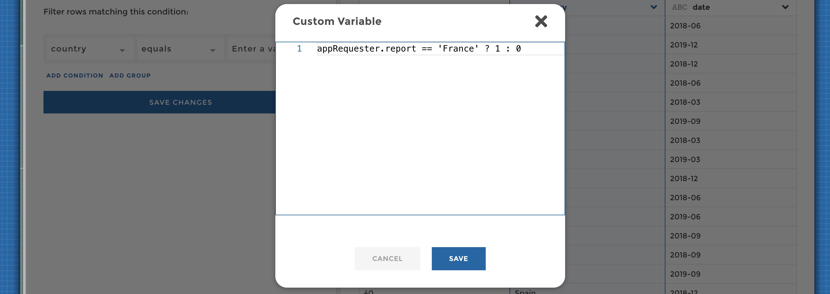
Advanced variable editor
In code mode the syntax looks like <variableScope>.<variableName>.
Here are the three variable scopes that you can use:
- For a global variable (a view or a date), the variable scope will be
appRequester - For a story variable, the variable scope will be
requestersManager - For a user variable, the variable scope will be
user
For the variables name:
- For a global variable,it will be either
report(for views) ordate(for dates) - For a story variable, it will be the name you gave to the requester when you configured it
- For a user variable, it will be the name of the user attribute. By
default, you can acces Toucan Toco attributes
groups(which value is the list of the Toucan user groups the user belongs to) andusername(the user login email). But you may expose some custom attributes derived from your dentity provider
Complete Object Mode
When defining a requester (on the home or in your stories), you have the
option to use all the columns of your underlying dataset. In such a
case, to access any of the column in your queries, the syntax looks like
<variableScope>.<variableName>.<someField>
So for example if you use views with this underlying dataset:
| city | country | region |
|---|---|---|
| Paris | France | Europe |
| Amsterdam | Netherlands | Europe |
| Boston | USA | North America |
| Toronto | Canada | North America |
You can use make your queries dynamic depending on either the city
(appRequesters.report.city), the country
(appRequesters.report.country) or the region
(appRequesters.report.region).
Ternary syntax: conditionals
You can use a powerful syntax allowing you to make a variable value depend on another. For example, let’s say that you want your variable to take the value 1 if some requester value is ‘FILTER ME’, else the variable should take the value 0.
Then you can write:
requestersManager.yourVariable == 'FILTER ME' ? 1 : 0
The syntax is
<condition to verify> ? <value if true> : <value if false>
You can use any other Javascript comparison operator like !=, >,
<, >=, <=…
Do not filter in some conditions: the use of ‘__VOID__’
In some (or lot of) cases, you may not want to apply some filtering based on the value of a variable. The most fequent use case is when you have “ALL” values in your requesters (“All countries”, “All products”…). The underlying data would look like this:
| country |
|---|
| All countries |
| France |
| Netherlands |
| USA |
| Canada |
Then in your queries, let’s say that you need to first filter your data before aggregating it. For any country selected, you want to apply a filter to keep only the country rows before aggregating. But when “All countries” is selected, you do not want to apply any filter as you want to aggregate all the countries rows.
So how to do that? In Toucan, you can use a special value, which is ‘__VOID__’. When a variable takes this value, it will just not be taken into account. So in ourt example it’s very useful because it allows to express exactly what we need with a ternary syntax (see section just above):
appRequesters.report === 'All countries' ? '__VOID__' : appRequesters.report
Meaning: if the value selected is “All countries”, then the variable should be ‘__VOID__’ and no filter will apply, else the variable should take the value selected (any country).
Variables in code mode
Note that if you do not use YouPrep™ and that you want to use variables
in code mode, you must add the variables delimiters <%= and %>
in your queries or chart configuration. It looks like this:
<%= appRequesters.report %>
See this detailed documention.
How to play with data requests in code mode
While editing a chart, you can select Data request editor (next to
Chart parameters) to display the data request editor.
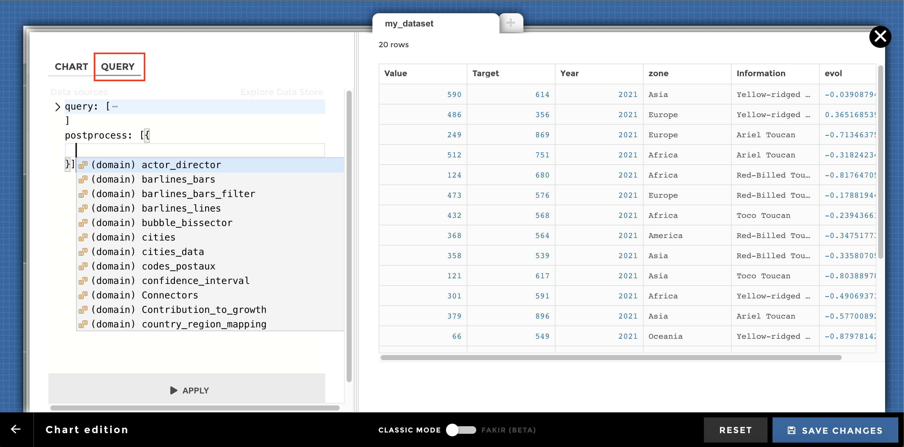
Data request editor
It is possible to do a little postprocess in the data request. This will allow you to do some massaging on the data. You can:
These functions can be found inside the utils/postprocess folder in toucan-data-sdk.
👉 You can use postprocess inside the data request editor at the same
level as the query block. Here is an example for a roll_up
process:
query:
  domain:'my_domain'
postprocess:[
  roll_up:
    levels : [0,1,2]
    groupby_vars: ['colA', colB]
    var_name: 'my_var_name'
]
👉 A post process can contain multiple steps, make sure to separate them
with a ,
postprocess:[
  roll_up:
    levels : [0,1,2]
    groupby_vars: ['colA', colB]
    var_name: 'my_var_name'
,
  argmax:
    column: 'year'
]
Postprocess: clean
add_missing_row
Add missing rows based on reference values.
postprocess:[
  add_missing_row:
    id_cols: ['Col_name_1', 'Col_name_2']
    reference_col: 'Reference_col_name'
    complete_index:[A, B, C]
    method: 'between'
    cols_to_keep: ['Col_name_3']
]
mandatory :
id_cols(list of str): names of the columns used to create each groupreference_col(str): name of the column used to identify missing rows
optional :
complete_index(list or dict):[A, B, C] a list of values used to add missing rows. It can also be a dict to declare a date range. By default, use all values of reference_col.method(str): by default all missing rows are added. The possible values are :"between": add missing rows having their value between min and max values for each group,"between_and_after": add missing rows having their value bigger than min value for each group."between_and_before": add missing rows having their value smaller than max values for each group.
cols_to_keep(list of str): name of other columns to keep, linked to the reference_col.
Input:
| id_cols | reference_col |
|---|---|
| 2016 | A |
| 2016 | B |
| 2016 | C |
| 2017 | A |
| 2017 | C |
data:
  query:
    domain: "my_domain"
  postprocess:[
    add_missing_row:
      id_cols: ['id_cols']
      reference_col: 'reference_col'
  ]
Output:
| id_cols | reference_col |
|---|---|
| 2016 | A |
| 2016 | B |
| 2016 | C |
| 2017 | A |
| 2017 | B |
| 2017 | C |
Input:
| id_cols | reference_col |
|---|---|
| 2016 | B |
| 2017 | C |
data:
  query:
    domain: "my_domain"
  postprocess:[
    add_missing_row:
      id_cols: ['id_cols']
      complete_index:['A', 'B', 'C']
      reference_col: 'reference_col'
  ]
Output:
| id_cols | reference_col |
|---|---|
| 2016 | A |
| 2016 | B |
| 2016 | C |
| 2017 | A |
| 2017 | B |
| 2017 | C |
cast
Change type of a column
postprocess: [
  cast:
    column: 'my_column'
    type: 'int'
]
mandatory :
column(str): name of the column to converttype(str): output type. It can be :"int": integer type"float": general number type"str": text type
optional :
new_column(str): name of the output column. By default thecolumnarguments is modified.
Input :
| Column 1 | Column 2 | Column 3 |
|---|---|---|
| ‘one’ | ‘2014’ | 30.0 |
| ‘two’ | 2015.0 | ‘1’ |
| 3.1 | 2016 | 450 |
postprocess: [
  cast:
    column: 'Column 1'
    type: 'str'
  cast:
    column: 'Column 2'
    type: 'int'
  cast:
    column: 'Column 3'
    type: 'float'
]
Output:
| Column 1 | Column 2 | Column 3 |
|---|---|---|
| ‘one’ | 2014 | 30.0 |
| ‘two’ | 2015 | 1.0 |
| ‘3.1’ | 2016 | 450.0 |
convert_datetime_to_str
- Convert a datetime object into string according to the format of your choice *
postprocess: [
  convert_datetime_to_str:
    column: 'my_date_column'
    format: 'my_format'
]
madatory:
column(str) : Name of the column to convert into stringformat(str) : Output format. Please use the following syntax : https://github.com/d3/d3-time-format#api-reference
optional :
new_column(str): name of the output column. By default thecolumnarguments is modified.
Input :
| label | value |
|---|---|
| France | 2017-03-22 15:16:00 |
| Europe | 2016-03-22 15:16:00 |
convert_datetime_to_str:
  column: 'value'
  format: '%Y-%m'
]
Output :
| label | value |
|---|---|
| France | 2017-03 |
| Europe | 2016-03 |
change_date_format
Change a date column from a format to an other
postprocess: [
  change_date_format:
    column: 'my_date_column'
    output_format: '%Y%-%m-%d'
]
madatory:
column(str) : Name of the column to convert into stringoutput_format(str) : Output format. Please use the following syntax : https://github.com/d3/d3-time-format#api-reference
optional :
new_column(str): name of the output column. By default thecolumnarguments is modified.input_format(str): Original date format ofcolumn. Please use the following syntax : https://github.com/d3/d3-time-format#api-reference
Input :
| label | date |
|---|---|
| France | 2017-03-22 |
| Europe | 2016-03-22 |
change_date_format:
  column: 'date'
  input_format: '%Y-%m-%d'
  output_format: '%Y-%m'
]
Output :
| label | date |
|---|---|
| France | 2017-03 |
| Europe | 2016-03 |
Input :
| label | date |
|---|---|
| France | 2017-03-22 |
| Europe | 2016-02-22 |
change_date_format:
  column: 'date'
  new_column: 'month'
  input_format: '%Y-%m-%d'
  output_format: '%B'
]
Output :
| label | date | month |
|---|---|---|
| France | 2017-03 | March |
| Europe | 2016-02 | February |
fillna
Will fill in missing values with a specific value.
data:
  query:
    domain: "my_domain"
  postprocess:[
    fillna:
      column: 'my_value'
      value: 0
  ]
mandatory :
column(str) : column name on which we want to replace missing values by another valuevalue: value replacing missing values
Input:
| variable | wave | year | my_value |
|---|---|---|---|
| toto | wave 1 | 2014 | 300 |
| toto | wave 1 | 2015 | |
| toto | wave 1 | 2016 | 450 |
data:
  query:
    domain: "my_domain"
  postprocess:[
    fillna:
      column: 'my_value'
      value: 0
  ]
Output:
| variable | wave | year | my_value |
|---|---|---|---|
| toto | wave 1 | 2014 | 300 |
| toto | wave 1 | 2015 | 0 |
| toto | wave 1 | 2016 | 450 |
If column doesn’t exist in the dataframe, it will be added with
value as value :
Input:
| variable | wave | year | my_value |
|---|---|---|---|
| toto | wave 1 | 2014 | 300 |
| toto | wave 1 | 2015 | |
| toto | wave 1 | 2016 | 450 |
data:
  query:
    domain: "my_domain"
  postprocess:[
    fillna:
      column: 'other_column'
      value: 50
  ]
Output:
| variable | wave | year | my_value | other_column |
|---|---|---|---|---|
| toto | wave 1 | 2014 | 300 | 50 |
| toto | wave 1 | 2015 | 50 | |
| toto | wave 1 | 2016 | 450 | 50 |
rename
Change the label of a value or a columns within your data source.
postprocess: [
  rename:
    values:
      'value_to_modify':
        'en': 'new_value'
        'fr': 'new_value'
    columns:
      'column_to_rename':
        'en': 'new_value'
        'fr': 'new_value'
]
⚠️ You have to rename in ‘en’ and ‘fr’ otherwise it will not work.
Note: The rename postprocess accepts a fallback_locale parameter
that will be used as a default locale if locale is not found in
translations.
Input :
| label | value |
|---|---|
| France | 100 |
| Europe wo France | 500 |
postprocess: [
rename:
    values:
    'Europe wo France':
      'en': 'Europe excl. France'
      'fr': 'Europe excl. France'
    columns:
    'value':
      'en': 'revenue'
      'fr': 'revenue'
]
Output :
| label | revenue |
|---|---|
| France | 100 |
| Europe excl. France | 500 |
Input :
| label | value |
|---|---|
| France | 100 |
| Europe wo France | 500 |
postprocess: [
rename:
    values:
    'Europe wo France':
      'en': 'Europe excl. France'
      'fr': 'Europe sauf. France'
    columns:
    'value':
      'en': 'revenue'
      'fr': 'revenus'
    locale: 'it'
    fallback_locale: 'en'
]
Output :
| label | revenue |
|---|---|
| France | 100 |
| Europe excl. France | 500 |
replace
Change the label of a value or a columns within your data source. (Similar to ``rename`` but does not have the notion of locale)
postprocess: [
  replace:
    column: "column_to_modify"
    new_column: "new_column"
    to_replace:
      "old_value": "new_value"
      "old_value_2": "new_value_2"
]
mandatory :
column(str): name of the column to modify.to_replace(dict): keys of this dict are old values pointing on substitute.
optional :
new_column(str): name of the output column. By default thecolumnarguments is modified.
Input :
| article | rating |
|---|---|
| book | 1 |
| puzzle | 3 |
| food | 5 |
We want to split the ratings in three categories: “good”, “average” and “poor”.
postprocess: [
  replace:
    column: "rating"
    new_column: "rating_category"  # create a new column with replaced data
    to_replace:
      1: "poor"
      2: "poor"
      3: "average"
      4: "good"
      5: "good"
]
Output :
| article | rating | rating_category |
|---|---|---|
| book | 1 | poor |
| puzzle | 3 | average |
| food | 5 | good |
Input :
| article | comment |
|---|---|
| book | I didnt recieve the book |
| puzzle | Couldnt acheive it, fuuuck |
| food | Fucking yummy! |
We fix some common orthographic mistakes using regular expressions (regex):
postprocess: [
  replace:
    column: "comment"
    to_replace:
      "recieve": "receive"
      "acheive": "achieve"
      "([fF])u+ck": "\g<1>*ck"  # censoring :o
    regex: true
]
Output :
| article | comment |
|---|---|
| book | I didnt receive the book |
| puzzle | Couldnt achieve it, f*ck |
| food | F*cking yummy! |
Postprocess : Filter
argmax and argmin
Keep in the dataframe a maximal (or minimal) value of a row.
👉 Query in the dataframe rows with latest (oldest) date.
postprocess:[
  argmax:
    column: 'my_column'
]
mandatory :
column: column name on which we want to keep the maximal (minimal) value
Input:
| variable | wave | year | value |
|---|---|---|---|
| toto | wave 1 | 2014 | 300 |
| toto | wave 1 | 2015 | 250 |
| toto | wave 1 | 2016 | 450 |
postprocess:[
  argmax:
    column: 'year'
]
Output:
| variable | wave | year | value |
|---|---|---|---|
| toto | wave 1 | 2016 | 450 |
Input:
| variable | wave | year | value |
|---|---|---|---|
| toto | wave 1 | 2014 | 300 |
| toto | wave 1 | 2015 | 250 |
| toto | wave 1 | 2016 | 450 |
postprocess:[
  argmin:
    column: 'year'
]
Output:
| variable | wave | year | value |
|---|---|---|---|
| toto | wave 1 | 2014 | 300 |
drop_duplicates
- Drop duplicate rows*
postprocess: [
  drop_duplicates:
    columns: ['col1', 'col2']
]
mandatory :
columns: columns to consider to identify duplicates (set to null to use all the columns)
Input:
| name | country | year |
|---|---|---|
| toto | France | 2014 |
| titi | England | 2015 |
| toto | France | 2014 |
| toto | France | 2016 |
postprocess: [
  drop_duplicates:
    columns: null
]
Output:
| name | country | year |
|---|---|---|
| toto | France | 2014 |
| titi | England | 2015 |
| toto | France | 2016 |
coffeescript postprocess: [ drop_duplicates: columns: ['name', 'country'] ]
Output:
| name | country | year |
|---|---|---|
| toto | France | 2014 |
| titi | England | 2015 |
query
Filter a dataset under a condition
👉 Similar to $match step in Mongo
postprocess:[
    query: 'value > 1'
]
Input:
| variable | wave | year | value |
|---|---|---|---|
| toto | wave 1 | 2014 | 300 |
| toto | wave 1 | 2015 | 250 |
| toto | wave 1 | 2015 | 100 |
| toto | wave 1 | 2016 | 450 |
postprocess:[
    query: 'value > 350'
]
Output:
| variable | wave | year | value |
|---|---|---|---|
| toto | wave 1 | 2016 | 450 |
postprocess:[
    query: 'year == 2015'
]
Output:
| variable | wave | year | value |
|---|---|---|---|
| toto | wave 1 | 2015 | 250 |
| toto | wave 1 | 2015 | 100 |
if else
Transform a part of your dataset according to certain conditions : a classic if… then… else… option
if_else:
  if: <query>
  then: <string, number, boolean or new postprocess>
  else: <string, number, boolean or new postprocess>
  new_column: <the new column name>
mandatory :
if(str): string representing the query to filter the data (same as the one used in the postprocess ‘query’) See pandas doc for more informationthen:- str, int, float: A row value to use for the new column
- dict or list of dicts: postprocesses functions to have more logic (see examples)
new_column(str): name of the column containing the result. optional :else: same as then but for the non filtered part. If not set, the non filtered part won’t have any values for the new column
Input :
| country | city | clean | the rating |
|---|---|---|---|
| France | Paris | -1 | 3 |
| Germany | Munich | 4 | 5 |
| France | Nice | 3 | 4 |
| Hell | HellCity | -10 | 0 |
  if_else:
    if: '`the rating` % 2 == 0'
    then:
      postprocess: 'formula'
      formula: '("the rating" + clean) / 2'
    else: 'Hey !'
    new_column: 'new'
]
Output:
| country | city | clean | the rating | new |
|---|---|---|---|---|
| France | Paris | -1 | 3 | Hey! |
| Germany | Munich | 4 | 5 | Hey! |
| France | Nice | 3 | 4 | 3.5 |
| Hell | HellCity | -10 | 0 | -5.0 |
top
Get the top or flop N results based on a column value. You can execute the selection on group columns
postprocess:[
  top:
      value: "column_name"
      limit: 10
      order: 'asc'
]
mandatory :
value(str): Name of the column name on which you will rank the results.limit(int): Number to specify the N results you want to retrieve from the sorted values.- Use a positive number x to retrieve the first x results.
- Use a negative number -x to retrieve the last x results.
optional :
order(str):"asc"or"desc"to sort by ascending ou descending order. By default :"asc".group(str, list of str): name(s) of columns on which you want to perform the group operation.
Input :
| variable | Category | value |
|---|---|---|
| lili | 1 | 50 |
| lili | 1 | 20 |
| toto | 1 | 100 |
| toto | 1 | 200 |
| toto | 1 | 300 |
| lala | 1 | 100 |
| lala | 1 | 150 |
| lala | 1 | 250 |
| lala | 2 | 350 |
| lala | 2 | 450 |
postprocess:[
  top:
    value: 'value'
    limit: 4
    order: 'asc'
]
Output:
| variable | Category | value |
|---|---|---|
| lala | 1 | 250 |
| toto | 1 | 300 |
| lala | 2 | 350 |
| lala | 2 | 450 |
Input :
| variable | Category | value |
|---|---|---|
| lili | 1 | 50 |
| lili | 1 | 20 |
| toto | 1 | 100 |
| toto | 1 | 200 |
| toto | 1 | 300 |
| lala | 1 | 100 |
| lala | 1 | 150 |
| lala | 1 | 250 |
| lala | 2 | 350 |
| lala | 2 | 450 |
postprocess:[
  top:
      group: ["Category"]
      value: 'value'
      limit: 2
      order: 'asc'
]
Output:
| variable | Category | value |
|---|---|---|
| lala | 1 | 250 |
| toto | 1 | 300 |
| lala | 2 | 350 |
| lala | 2 | 450 |
top_group
Get the results based on a column value and a function that aggregates the input and keeps only the N top or flop groups. The result is composed by all lines corresponding to the top groups
postprocess: [
  top_group:
    "group": ["Category"]
    "value": 'value'
    "aggregate_by": ["variable"]
    "limit": 2
    "order": "desc"
]
mandatory :
value(str): Name of the column name on which you will rank the results.limit(int): Number to specify the N results you want to retrieve from the sorted values.- Use a positive number x to retrieve the first x results.
- Use a negative number -x to retrieve the last x results.
aggregate_by(list of str)): name(s) of columns you want to aggregate
optional :
order(str):"asc"or"desc"to sort by ascending ou descending order. By default :"asc".group(str, list of str): name(s) of columns on which you want to perform the group operation.function: Function to use to group over the group column
Input :
| variable | Category | value |
|---|---|---|
| lili | 1 | 50 |
| lili | 1 | 20 |
| toto | 1 | 100 |
| toto | 1 | 200 |
| toto | 1 | 300 |
| lala | 1 | 100 |
| lala | 1 | 150 |
| lala | 1 | 250 |
| lala | 2 | 350 |
| lala | 2 | 450 |
postprocess: [
  top_group:
    "group": ["Category"]
    "value": 'value'
    "aggregate_by": ["variable"]
    "limit": 2
    "order": "desc"
]
Output :
| variable | Category | value |
|---|---|---|
| toto | 1 | 100 |
| toto | 1 | 200 |
| toto | 1 | 300 |
| lala | 1 | 100 |
| lala | 1 | 150 |
| lala | 1 | 250 |
| lala | 2 | 350 |
| lala | 2 | 450 |
filter_by_date
Filter out a dataset according to a date range specification
postprocess:[
  filter_by_date:
      start: "2018-01-01"
      stop: "2018-01-04"
      date_format: "%Y-%m-%d"
]
mandatory :
date_col: the name of the dataframe’s column to filter on
optional :
date_format: expected date format in columndate_col(default is%Y-%m-%d)start: if specified, lower bound (included) of the date rangestop: if specified, upper bound (excluded) of the date rangeatdate: if specified, the exact date we’re filtering on
Even though start, stop and atdate are individually not
required, you must use one of the following combinations to specify
the date range to filter on:
atdate: keep all rows matching this date exactly,start: keep all rows matching this date onwards (bound included),stop: keep all rows matching dates before this one (bound excluded),startandstop: keep all rows betweenstart(included) andstop(excluded).
Besides standard date formats, you can also:
- use the following symbolic names (
TODAY,YESTERDAYandTOMORROW), - use offsets with either
(datestr) + OFFSETor(datestr) - OFFSETsyntax. In this case,OFFSETmust be understable bypandas.Timedelta(cf. http://pandas.pydata.org/pandas-docs/stable/timedeltas.html) anddatestrmust be wrapped with parenthesis (e.g.(2018-01-01) + 2d), - use a combination of both symbolic names and offsets (e.g.
(TODAY) + 2d).
Input :
| date | value |
|---|---|
| 2018-01-28 | 0 |
| 2018-01-28 | 1 |
| 2018-01-29 | 2 |
| 2018-01-30 | 3 |
| 2018-01-31 | 4 |
| 2018-02-01 | 5 |
| 2018-02-02 | 6 |
postprocess:[
  filter_by_date:
    date_col: 'date'
    date_fmt: '%Y-%m-%d'
    start: '2018-01-31'
]
Output:
| date | value |
|---|---|
| 2018-01-31 | 4 |
| 2018-02-01 | 5 |
| 2018-02-02 | 6 |
Input :
| date | value |
|---|---|
| 2018-01-28 | 0 |
| 2018-01-28 | 1 |
| 2018-01-29 | 2 |
| 2018-01-30 | 3 |
| 2018-01-31 | 4 |
| 2018-02-01 | 5 |
| 2018-02-02 | 6 |
postprocess:[
  filter_by_date:
    date_col: 'date'
    date_fmt: '%Y-%m-%d'
    start: '(2018-01-29) + 2days'
]
Output:
| date | value |
|---|---|
| 2018-01-31 | 4 |
| 2018-02-01 | 5 |
| 2018-02-02 | 6 |
Input :
| date | value |
|---|---|
| 2018-01-28 | 0 |
| 2018-01-28 | 1 |
| 2018-01-29 | 2 |
| 2018-01-30 | 3 |
| 2018-01-31 | 4 |
| 2018-02-01 | 5 |
| 2018-02-02 | 6 |
postprocess:[
  filter_by_date:
    date_col: 'date'
    date_fmt: '%Y-%m-%d'
    start: '2018-01-29'
    stop: '2018-02-01'
]
Output:
| date | value |
|---|---|
| 2018-01-29 | 2 |
| 2018-01-30 | 3 |
| 2018-01-31 | 4 |
Input :
| date | value |
|---|---|
| 2018-01-28 | 0 |
| 2018-01-28 | 1 |
| 2018-01-29 | 2 |
| 2018-01-30 | 3 |
| 2018-01-31 | 4 |
| 2018-02-01 | 5 |
| 2018-02-02 | 6 |
postprocess:[
  filter_by_date:
    date_col: 'date'
    date_fmt: '%Y-%m-%d'
    stop: '2018-02-01'
]
Output:
| date | value |
|---|---|
| 2018-01-28 | 0 |
| 2018-01-28 | 1 |
| 2018-01-29 | 2 |
| 2018-01-30 | 3 |
| 2018-01-31 | 4 |
Input :
| date | value |
|---|---|
| 2018-01-28 | 0 |
| 2018-01-28 | 1 |
| 2018-01-29 | 2 |
| 2018-01-30 | 3 |
| 2018-01-31 | 4 |
| 2018-02-01 | 5 |
| 2018-02-02 | 6 |
postprocess:[
  filter_by_date:
    date_col: 'date'
    date_fmt: '%Y-%m-%d'
    atdate: '2018-01-28'
]
Output:
| date | value |
|---|---|
| 2018-01-28 | 0 |
| 2018-01-28 | 1 |
Input :
| date | value |
|---|---|
| 2018-01-28 | 0 |
| 2018-01-28 | 1 |
| 2018-01-29 | 2 |
| 2018-01-30 | 3 |
| 2018-01-31 | 4 |
| 2018-02-01 | 5 |
| 2018-02-02 | 6 |
postprocess:[
  filter_by_date:
    date_col: 'date'
    date_fmt: '%Y-%m-%d'
    start: 'TODAY'
]
Output:
| date | value |
|---|---|
| 2018-01-29 | 2 |
| 2018-01-30 | 3 |
| 2018-01-31 | 4 |
| 2018-02-01 | 5 |
| 2018-02-02 | 6 |
Input :
| date | value |
|---|---|
| 2018-01-28 | 0 |
| 2018-01-28 | 1 |
| 2018-01-29 | 2 |
| 2018-01-30 | 3 |
| 2018-01-31 | 4 |
| 2018-02-01 | 5 |
| 2018-02-02 | 6 |
postprocess:[
  filter_by_date:
    date_col: 'date'
    date_fmt: '%Y-%m-%d'
    start: '(TODAY) + 2d'
    stop: '(TODAY) + 2d'
]
Output:
| date | value |
|---|---|
| 2018-01-28 | 0 |
| 2018-01-28 | 1 |
| 2018-01-29 | 2 |
| 2018-01-30 | 3 |
Postprocess : Aggregate
groupby
Aggregate values by groups.
postprocess: [
  groupby:
    group_cols: ['colname_1', 'colname_2']
    aggregations:
      'value_1': 'sum'
      'value_2': 'mean'
]
mandatory :
group_cols(list of str): name(s) of columns used to group dataaggregations(dict) : dictionary of values columns to group as keys and aggregation function to use as values. Available aggregation functions:'sum''mean''median''prod'(product)'std'(standard deviation)'var'(variance)
Input:
| ENTITY | YEAR | VALUE_1 | VALUE_2 |
|---|---|---|---|
| A | 2017 | 10 | 3 |
| A | 2017 | 20 | 1 |
| A | 2018 | 10 | 5 |
| A | 2018 | 30 | 4 |
| B | 2017 | 60 | 4 |
| B | 2017 | 40 | 3 |
| B | 2018 | 50 | 7 |
| B | 2018 | 60 | 6 |
postprocess: [
  groupby:
    group_cols: ['ENTITY', 'YEAR']
    aggregations:
      'VALUE_1': 'sum'
      'VALUE_2': 'mean'
]
Output:
| ENTITY | YEAR | VALUE_1 | VALUE_2 |
|---|---|---|---|
| A | 2017 | 30 | 2.0 |
| A | 2018 | 40 | 4.5 |
| B | 2017 | 100 | 3.5 |
| B | 2018 | 110 | 6.5 |
roll_up
Creates aggregates following a given hierarchy.
postprocess:[
  roll_up:
    levels: ["col_name_1", "col_name_2"]
    groupby_vars: ["value_1", "value_2"]
    extra_groupby_cols: # (list(str)) optional: other columns used to group in each level.
    var_name: "output_var"
    value_name:  "output_value"
    agg_func: "sum"
    drop_levels: ["level_1", "level_2"]
]
mandatory :
levels(list of str): name of the columns composing the hierarchy (from the top to the bottom level).groupby_vars(list of str): name of the columns with value to aggregate.extra_groupby_cols(list of str) optional: other columns used to group in each level.
optional :
var_name(str) : name of the result variable column. By default,“type”.value_name(str): name of the result value column. By default,“value”.agg_func(str): name of the aggregation operation. By default,“sum”.drop_levels(list of str): the names of the levels that you may want to discard from the output.
Input :
| Region | City | Population |
|---|---|---|
| Idf | Panam | 200 |
| Idf | Antony | 50 |
| Nord | Lille | 20 |
postprocess:[
  roll_up:
    levels: ["Region", "City"]
    groupby_vars: "Population"
]
Output:
| Region | City | Population | value | type |
|---|---|---|---|---|
| Idf | Panam | 200 | Panam | City |
| Idf | Antony | 50 | Antony | City |
| Nord | Lille | 20 | Lille | City |
| Idf | Nan | 250 | Idf | Region |
| Nord | Nan | 20 | Nord | Region |
combine_columns_aggregation
Aggregates data based on all possible combinations of values found in specified columns.
postprocess:[
  combine_columns_aggregation:
    id_cols: ['Col_name_1', "Col_name_2"]
    cols_for_combination:
      'Col_name_3': 'All_3',
      'Col_name_4': 'All_4'
    agg_func: 'sum'
]
mandatory :
id_cols(list of str): name of the columns used to create each groupcols_for_combination(dict): name of the input columns for combination as key and their output label as value
optional :
agg_func(string or dict or list): Use for aggregating the data. By default"sum"
Initial data:
| Year | City | Category | Value |
|---|---|---|---|
| 2017 | Paris | A | 5 |
| Nantes | A | 4 | |
| Paris | B | 7 | |
| 2016 | Nantes | A | 10 |
postprocess:[
  combine_columns_aggregation:
    id_cols: ['Year']
    cols_for_combination:
      'City': 'All Cities'
      'Category': 'All'
]
Output:
| Year | City | Category | Value |
|---|---|---|---|
| 2017 | Paris | A | 5 |
| Nantes | A | 4 | |
| Paris | B | 7 | |
| All Cities | A | 9 | |
| All Cities | B | 7 | |
| Nantes | All | 4 | |
| Paris | All | 12 | |
| All Cities | All | 16 | |
| 2016 | Nantes | A | 10 |
| All Cities | A | 10 | |
| Nantes | All | 10 | |
| All Cities | All | 10 |
compute_fill_by_group
Gives the result of a groupby with a ffill without the performance issue. The method ffill propagate last valid value forward to next values.
postprocess:[
  compute_ffill_by_group:
    id_cols: ["id_cols"]
    reference_cols: ["reference_cols"]
    value_col: ["value_col"]
]
mandatory :
id_cols(str or list of str): name(s) of the columns used to create each group.reference_cols(str or list of str): name (s)of the columns used to sort.value_col(str or list of str): name(s) of the columns to fill.
Initial data:
| id_cols | reference_cols | value_col |
|---|---|---|
| A | 1 | 2 |
| A | 2 | 5 |
| A | 3 | null |
| B | 1 | null |
| B | 2 | 7 |
postprocess:[
  compute_ffill_by_group:
    id_cols: "id_cols"
    reference_cols: "reference_cols"
    value_col: "value_col"
]
Output:
| id_cols | reference_cols | value_col |
|---|---|---|
| A | 1 | 2 |
| A | 2 | 5 |
| A | 3 | 5 |
| B | 1 | null |
| B | 2 | 7 |
Postprocess : Transform Structure
melt
A melt will transform a dataset by creating a column “variable” and a column “value”. This function is useful to transform a dataframe into a format where one or more columns are identifier variables, while all other columns, considered measured variables (value_vars), are “unpivoted” to the row axis, leaving just two non-identifier columns, ``”variable”`` and ``”value”``.
postprocess: [
  melt:
    id: ['my_column_1', 'my_colum_2']
    value: ['info_1', 'info_2', 'info_3']
    dropna: true
]
mandatory :
id(list of str): names of the columns that must be kept in column.value(list of str): names of the columns that will be transformed in long format (in rows).
optional :
dropna(boolean): It allows you to drop missing values. By default :true
Input :
| my_label | my_value | my_column_1 | my_column_2 | info_1 | info_2 | info_3 |
|---|---|---|---|---|---|---|
| toto | 10 | S45 | Lalaland | 10 | 20 | None |
postprocess: [
  melt:
    id: ['my_label', 'my_value' 'my_column_1', 'my_colum_2']
    value: ['info_1', 'info_2', 'info_3']
    dropna: true
]
Output :
| my_label | my_value | my_column_1 | my_column_2 | variable | value |
|---|---|---|---|---|---|
| toto | 10 | S45 | Lalaland | info_1 | 10 |
| toto | 10 | S45 | Lalaland | info_2 | 20 |
Input :
| my_label | my_value | my_column_1 | my_column_2 | info_1 | info_2 | info_3 |
|---|---|---|---|---|---|---|
| toto | 10 | S45 | Lalaland | 10 | 20 | None |
postprocess: [
  melt:
    id: ['my_column_1', 'my_colum_2']
    value: ['info_1', 'info_2', 'info_3']
]
Output :
| my_label | my_value | my_column_1 | my_column_2 | variable | value |
|---|---|---|---|---|---|
| toto | 10 | S45 | Lalaland | info_1 | 10 |
| toto | 10 | S45 | Lalaland | info_2 | 20 |
| toto | 10 | S45 | Lalaland | info_3 | None |
pivot
Reverse operation of melting. Useful for configuring evolution
postprocess:[
    pivot:
        index: ['variable','wave']
        column: 'year'
        value: 'value'
]
mandatory :
index(list): names of index columns.column(str): column name to pivot onvalue(str): column name containing the value to fill the pivoted df
Input :
| variable | wave | year | value |
|---|---|---|---|
| toto | wave 1 | 2014 | 300 |
| toto | wave 1 | 2015 | 250 |
| toto | wave 1 | 2016 | 450 |
postprocess:[
    pivot:
        index: ['variable','wave']
        column: 'year'
        value: 'value'
]
Output:
| variable | wave | 2014 | 2015 | 2015 |
|---|---|---|---|---|
| toto | wave 1 | 300 | 250 | 450 |
pivot_by_group
Pivot a dataframe by group of variables.
postprocess:[
  pivot_by_group :
    id_cols: ['type']
    variable: 'variable'
    value: 'montant'
    new_columns: ['value', 'variation']
    groups:
      'Group 1' : ['var1', 'var1_evol']
      'Group 2' : ['var2', 'var2_evol']
  ]
mandatory :
variable(str): name of the column used to create the groups.value(str): name of the column containing the value to fill the pivoted df.new_columns(list of str): names of the new columns.groups(dict): names of the groups with their corresponding variables. ⚠️ The list of variables has the same order thannew_columns
optional :
id_cols(list of str) : names of other columns to keep, defaultNone.
Input
| type | variable | montant |
|---|---|---|
| A | var1 | 5 |
| A | var1_evol | 0.3 |
| A | var2 | 6 |
| A | var2_evol | 0.2 |
postprocess:[
  pivot_by_group :
    id_cols: ['type']
    variable: 'variable'
    value: 'montant'
    new_columns: ['value', 'variation']
    groups:
      'Group 1' : ['var1', 'var1_evol']
      'Group 2' : ['var2', 'var2_evol']
  ]
Output
| type | variable | value | variation |
|---|---|---|---|
| A | Group 1 | 5 | 0.3 |
| A | Group 2 | 6 | 0.2 |
sort
Sort the data by the value in specified columns.
postprocess: [
  sort:
    columns: ["my_column1", "my_column2"]
    order: 'asc'
]
mandatory :
columns(str of list of str): name(s) the columns on which you want to sort.group(str, list of str): name(s) of columns on which you want to perform the group operation.
Input:
| variable | value |
|---|---|
| A | 220 |
| B | 200 |
| C | 300 |
| D | 100 |
postprocess:[
  sort:
      columns: ['variable']
      order: 'asc'
]
Output :
| variable | value |
|---|---|
| D | 100 |
| B | 200 |
| A | 220 |
| C | 300 |
two_values_melt
Transforms one or multiple columns into rows. Unlike melt function (pandas), two value columns can be returned by the function. For example, an evolution column and a price column.
postprocess:[
  two_values_melt:
    first_value_vars: ["avg", "total"]
    second_value_vars: ["evo_avg", "evo_total"]
    var_name: "type"
    value_name: "value"
]
mandatory :
first_value_vars(list of str): name of the columns corresponding to the first returned value columnsecond_value_vars(list of str): name of the columns corresponding to the second returned value columnvar_name(str): name of the column containing values in first_value_varsvalue_name(str): suffix of the two value columns (suffix_first / suffix_second)
Input :
| Region | avg | total | evo_avg | evo_total |
|---|---|---|---|---|
| A | 50 | 100 | 1 | 4 |
| B | 40 | 250 | 2 | 5 |
postprocess:[
  two_values_melt:
    first_value_vars: ["avg", "total"]
    second_value_vars: ["evo_avg", "evo_total"]
    var_name: "type"
    value_name: "value"
]
Output:
| Region | type | value_first | value_second |
|---|---|---|---|
| A | avg | 50 | 1 |
| A | total | 100 | 4 |
| B | avg | 40 | 2 |
| B | avg | 250 | 5 |
waterfall
This postprocess step simplify the data preparation for waterfall charts configuration.
postprocess:[
  waterfall:
    upperGroup:
      id: '<col>' # name of the column containing upperGroups unique IDs
      label: '<col>'  # name of the column containing text displayed under each upperGroups bars (not required, default on id)
      groupsOrder: '<col>'  # name of the column used for ordering of upperGroups (not requiered)
    insideGroup:
      id: '<col>'
      label: '<col>'
      groupOrder: '<col>'
    date: '<col>' # name of the column containing the id of the period of each lines
    value: '<col>' # name of the column containing the vaue for each lines
    start:
      label: '<value>' # text displayed under the first column
      id: '<value>' # value that identifies lines of the first period in the date column
    end:
      label: '<value>'
      id: '<value>'
    breakdown: [list of filter labels]
]
Input:
| product_id | played | date | ord | category_id | category_name |
|---|---|---|---|---|---|
| super clap | 12 | t1 | 1 | clap | Clap |
| clap clap | 1 | t1 | 10 | clap | Clap |
| tac | 1 | t1 | 1 | snare | Snare |
| super clap | 10 | t2 | 1 | clap | Clap |
| tac | 100 | t2 | 1 | snare | Snare |
| bom | 1 | t2 | 1 | tom | Tom |
postprocess:[
  waterfall:
    upperGroup:
      id: 'category_id'
      label: 'category_name'
    insideGroup:
      id: 'product_id'
      groupsOrder: 'ord'
    date: 'date'
    value: 'played'
    start:
      label: 'Trimestre 1'
      id: 't1'
    end:
      label: 'Trimester 2'
      id: 't2'
]
Output:
| value | label | variation | groups | type | order |
|---|---|---|---|---|---|
| 14 | Trimestre 1 | NaN | NaN | NaN | NaN |
| -3 | Clap | -0.230769 | clap | parent | NaN |
| -2 | super clap | -0.166667 | clap | child | 1 |
| -1 | clap clap | -1 | clap | child | 10 |
| 99 | Snare | 99 | snare | parent | NaN |
| 99 | tac | 99 | snare | child | 1 |
| 1 | Tom | inf | tom | parent | NaN |
| 1 | bom | inf | tom | child | 1 |
| 111 | Trimester 2 | NaN | NaN | NaN | NaN |
Postprocess : Compute
add_aggregation_columns
Add aggregation columns
postprocess: [
  add_aggregation_columns:
    group_cols: ['colname_1', 'colname_2']
    aggregations:
      new_col1:
        value_1: 'sum'
      new_col2:
        value_2: 'mean'
]
group_cols(list of str): name(s) of columns used to group dataaggregations(dict of dict): dictionary mapping the new columns and the corresponding aggregation dictionary. An aggregation dictionary is a dictionary with one key - the column you want to aggregate - and one value - the aggregation function amongstsum,max,min,mean,median,prod(product),std(standard deviation),var(variance)…
Input:
| ENTITY | YEAR | VALUE_1 | VALUE_2 |
|---|---|---|---|
| A | 2017 | 10 | 3 |
| A | 2017 | 20 | 1 |
| A | 2018 | 10 | 5 |
| A | 2018 | 30 | 4 |
| B | 2017 | 60 | 4 |
| B | 2017 | 40 | 3 |
| B | 2018 | 50 | 7 |
| B | 2018 | 60 | 6 |
postprocess: [
  add_aggregation_columns:
    group_cols: ['ENTITY', 'YEAR']
    aggregations:
      sum_value1:
        VALUE_1: 'sum'  # sum of `VALUE_1` put in `sum_value1` column
      max_value1:
        VALUE_1: 'max'  # max of `VALUE_1` put in `max_value1` column
      mean_value2:
        VALUE_2: 'mean'  # mean of `VALUE_2` put in `mean_value2` column
]
Output:
| ENTITY | YEAR | VALUE_1 | VALUE_2 | sum_value1 | max_value1 | mean_value2 |
|---|---|---|---|---|---|---|
| A | 2017 | 10 | 3 | 30 | 20 | 2.0 |
| A | 2017 | 20 | 1 | 30 | 20 | 2.0 |
| A | 2018 | 10 | 5 | 40 | 30 | 4.5 |
| A | 2018 | 30 | 4 | 40 | 30 | 4.5 |
| B | 2017 | 60 | 4 | 100 | 60 | 3.5 |
| B | 2017 | 40 | 3 | 100 | 60 | 3.5 |
| B | 2018 | 50 | 7 | 110 | 60 | 6.5 |
| B | 2018 | 60 | 6 | 110 | 60 | 6.5 |
compute_cumsum
Return a cumsum by group.
postprocess:[
  compute_cumsum:
    id_cols: #(list): name of the columns used to create each group..
    reference_cols: # (list): name of the columns used to order the cumsum.
    value_cols: # (list): name of the columns to cumsum.
    new_value_cols: # (list): name of th new columns with the cumsum.
    cols_to_keep: # (list) optional: other columns to keep in the dataframe. This option can be used if there is only one row by group identify with the columns id_cols and reference_cols
]
mandatory :
id_cols(list of str): names of the columns used to create each group..reference_cols(list of str): names of the columns used to order the cumsum.value_cols(list of str): names of the columns to cumsum.new_value_cols(list of str): names of th new columns with the cumsum.
optional :
cols_to_keep(list) : other columns to keep in the dataframe. This option can be used if there is only one row by group identify with the columns id_cols and reference_cols
Tips For an aggregation YearToDate, the column DATE is the
reference column and the column YEAR is an id column.
Input :
| Year | Date | Value |
|---|---|---|
| 2017 | 01/01/2017 | 1 |
| 02/01/2017 | 1 | |
| 03/01/2017 | 1 | |
| 2016 | 01/01/2017 | 1 |
| 02/01/2017 | 2 |
Configuration:
postprocess:[
  compute_cumsum:
    id_cols: ["Year"]
    reference_cols: ["Date"]
    value_cols: ["Value"]
    new_value_cols: ["Cumsum"]
]
Output:
| Year | Date | Value | Cumsum |
|---|---|---|---|
| 2017 | 01/01/2017 | 1 | 1 |
| 02/01/2017 | 1 | 2 | |
| 03/01/2017 | 1 | 3 | |
| 2016 | 01/01/2017 | 1 | 1 |
| 02/01/2017 | 2 | 3 |
absolute_values
Absolute value of each value of a column
postprocess:[
  absolute_values:
    column: 'my_numbers'
    new_column: 'my_positive_numbers'
]
mandatory :
column(str): name of the column
optional :
new_column(str): name of the result column with absolute values. If not set,columnwill be replaced.
Input :
| Values |
|---|
| 1.357 |
| 1.24 |
| -0.589 |
| -2 |
postprocess:[
  absolute_values:
    column: 'Values'
    new_column: 'Positive'
]
Output:
| Values | Positive |
|---|---|
| 1.357 | 1.357 |
| 1.24 | 1.24 |
| -0.589 | 0.589 |
| -2 | 2 |
round_values
Round each value of a column
postprocess:[
  round_values:
    column: 'my_numbers'
    decimals: 2
    new_column: 'my_numbers_rounded'
]
mandatory :
column(str): name of the columndecimals(int): number of decimals
optional :
new_column(str): name of the result column with rounded values. If not set,columnwill be replaced.
Input :
| Values |
|---|
| 1.357 |
| 1.24 |
| -0.589 |
| -2 |
postprocess:[
  round_values:
    column: 'Values'
    decimal: 1
    new_column: 'Rounded'
]
Output:
| Values | Rounded |
|---|---|
| 1.357 | 1.3 |
| 1.24 | 1.2 |
| -0.589 | -0.6 |
| -2 | -2 |
formula
Execute basics math operations on columns
postprocess:[
  formula:
    new_column: 'diff'
    formula: 'MyFirstColumn-MySecondColumn'
]
mandatory :
new_column(str): name of the output columnformula(str): Operation on column. Use name of column and special character :- “
+” for addition - “
-” for substration - “
*” for multiplication - “
/” for division
- “
Input :
| variable | valueA | valueB | valueC |
|---|---|---|---|
| toto | 20 | 100 | 10 |
| toto | 30 | 200 | 10 |
| toto | 10 | 300 | 10 |
postprocess:[
  formula:
    new_column: 'valueD'
    formula: '(valueB + valueA ) / valueC'
]
Output:
| variable | valueA | valueB | valueC | valueD |
|---|---|---|---|---|
| toto | 20 | 100 | 10 | 12 |
| toto | 30 | 200 | 10 | 23 |
| toto | 10 | 300 | 10 | 31 |
Input :
| variable | valueA | valueB | valueC |
|---|---|---|---|
| toto | 20 | 100 | 10 |
| toto | 30 | 200 | 10 |
| toto | 10 | 300 | 10 |
postprocess:[
  formula:
    new_column: 'valueD'
    formula: 'valueB + valueA  / valueC'
]
Output:
| variable | valueA | valueB | valueC | valueD |
|---|---|---|---|---|
| toto | 20 | 100 | 10 | 102 |
| toto | 30 | 200 | 10 | 203 |
| toto | 10 | 300 | 10 | 301 |
You also can use number in formula :
Input :
| variable | valueA | valueB |
|---|---|---|
| toto | 20 | 100 |
| toto | 30 | 200 |
| toto | 10 | 300 |
postprocess:[
  formula:
    new_column: 'valueA'
    formula: 'valueA/10'
]
Output:
| variable | valueA | valueB |
|---|---|---|
| toto | 2 | 100 |
| toto | 3 | 200 |
| toto | 1 | 300 |
compute_evolution_by_criteria
This function answers the question: how has a value changed compare to a specific value ?
postprocess:[
  compute_evolution_by_criteria:
    id_cols: #(list(str)): name of the columns used to create each group..
    value_col: # (str) : name of the column containing the value to compare
    compare_to: # (str) : the query identifying a specific set of values for comparison.
    method: # (str) optional: either abs for absolute values or pct for the evolution in percentage of previous value
    offseted_suffix: # (str) optional: suffix of the offseted column. By default, _offseted.
    evolution_col_name: # (str) optional: name given to the evolution column. By default, evolution_computed.
    raise_duplicate_error: # (bool) optional: raise an error - if set to True - or warning - if set to False- when the dataframe has duplicated values with the given id_cols.
    format: 'df' # Do not change it !!!
]
Input :
| id_cols | value_col | month |
|---|---|---|
| A | 100 | 1 |
| 250 | 12 | |
| B | 300 | 1 |
| 200 | 12 |
Configuration:
postprocess:[
  compute_evolution_by_criteria:
    id_cols: "id_cols"
    value_col: "value_col"
    compare_to: "month==12"
]
Output:
| id_cols | value_col | month | value_offseted | evolution_computed |
|---|---|---|---|---|
| A | 100 | 1 | 250 | -150 |
| 250 | 12 | 250 | 0 | |
| B | 300 | 1 | 200 | 100 |
| 200 | 12 | 200 | 0 |
compute_evolution_by_frequency
This function answers the question: how has a value changed on a weekly, monthly, yearly basis ?
postprocess:[
  compute_evolution_by_frequency:
    id_cols: # (list(str)): name of the columns used to create each group.
    date_col: # (str) : name of the column containing the date.
    value_col: # (str) : name of the column containing the value to compare
    freq: #(int/pd.DateOffset/pd.Serie/dict): the frequency at which we calculate evolutions (anything that can be added to the pd.Serie present in date_col). By default, 1.
      years: 1
      days: 1
      months: 1
    method: # (str) optional: either abs for absolute values or pct for the evolution in percentage of previous value
    offseted_suffix: #(str) optional: suffix of the offseted column. By default, _offseted.
    evolution_col_name: # (str) optional: name given to the evolution column. By default, evolution_computed.
    missing_date_as_zero: # (boolean) optional: add missing date with zero value.
    raise_duplicate_error: # (bool) optional: raise an error - if set to True - or a warning - if set to False- when the dataframe has duplicated values with the given id_cols.
    format: 'df' # Do not change it !!!
]
Tips
When you use missing_date_as_zero=False and format: 'df', since
both the original dataframe index and the evoluiton serie index are
matching, the result of the function can be add as a new column on the
original dataframe.
Input :
| id_cols | value_col | date_col |
|---|---|---|
| A | 20 | 2010 |
| 7 | 2011 | |
| B | 200 | 2010 |
| 220 | 2011 | |
| C | 100 | 2011 |
Configuration:
postprocess:[
  compute_evolution_by_frequency:
    id_cols: "id_cols"
    date_col: "date_col"
    value_col: "value_col"
]
Output:
| id_cols | value_col | date_col | evolution |
|---|---|---|---|
| A | 20 | 2010 | null |
| 7 | 2011 | -13 | |
| B | 200 | 2010 | null |
| 220 | 2011 | 20 | |
| C | 100 | 2011 | null |
percentage
Creates a new column, which is the percentage of a column regarding of the groupby logic
postprocess:[
  percentage:
    new_column: 'number_percentage'
    column: 'number'
    group_cols: ['sport']
]
mandatory :
column: name of the desired column you need percentage on
optional :
group_cols(list): names of columns for the groupby logicnew_column(str): name of the output column. By default thecolumnarguments is modified.
Input:
| gender | sport | number |
|---|---|---|
| male | bicycle | 17 |
| female | basketball | 17 |
| male | basketball | 3 |
| female | football | 7 |
| female | running | 30 |
| male | running | 20 |
| male | football | 21 |
| female | bicycle | 17 |
postprocess:[
  percentage:
    new_column: 'number_percentage'
    column: 'number'
    group_cols: ['sport']
]
Output:
| gender | sport | number | number_percentage |
|---|---|---|---|
| male | bicycle | 17 | 50.0 |
| female | basketball | 17 | 85.0 |
| male | basketball | 3 | 15.0 |
| female | football | 7 | 25.0 |
| female | running | 30 | 60.0 |
| male | running | 20 | 40.0 |
| male | football | 21 | 75.0 |
| female | bicycle | 17 | 50.0 |
rank
Create rank column(s) based on numeric values to be ranked. Independent ranking can be performed for different groups.
postprocess:[
  rank :
    value_cols: ['VALUE_1', 'VALUE_2']
    group_cols: ['ENTITY', 'YEAR']
    rank_cols_name: ['RANK_1', 'RANK_2']
  ]
mandatory :
value_cols(str or list(str)): name(s) of the columns usedgroup_cols(str or list(str), optionnal): name(s) of the column(s) used to create each group inside which independent ranking needs to be appliedrank_cols_names(str or list(str), optionnal): the names of the added ranking columns. If not filled in, the ranking will be named after the value_cols with a ‘_rank’ suffix
optional :
method(str): method to use when encountering equal values:'min'(default): lowest rank in group'max': highest rank in group'average': average rank of group'first': ranks assigned in order the values appear in the series'dense': like ‘min’, but rank always increases by 1 between groups
ascending(bool):true(default) orfalsewhether the rank should be determined based on ascending or descending order respectively
Input :
| ENTITY | YEAR | VALUE_1 | VALUE_2 |
|---|---|---|---|
| A | 2017 | 10 | 3 |
| A | 2017 | 20 | 1 |
| A | 2018 | 10 | 5 |
| A | 2018 | 30 | 4 |
| B | 2017 | 60 | 4 |
| B | 2017 | 40 | 3 |
| B | 2018 | 50 | 7 |
| B | 2018 | 50 | 6 |
postprocess:[
  rank :
    value_cols: 'VALUE_1'
  ]
Output :
| ENTITY | YEAR | VALUE_1 | VALUE_2 | VALUE_1_rank |
|---|---|---|---|---|
| A | 2017 | 10 | 3 | 1 |
| A | 2017 | 20 | 1 | 3 |
| A | 2018 | 10 | 5 | 1 |
| A | 2018 | 30 | 4 | 4 |
| B | 2017 | 60 | 4 | 8 |
| B | 2017 | 40 | 3 | 5 |
| B | 2018 | 50 | 7 | 6 |
| B | 2018 | 50 | 6 | 6 |
Input :
| ENTITY | YEAR | VALUE_1 | VALUE_2 |
|---|---|---|---|
| A | 2017 | 10 | 3 |
| A | 2017 | 20 | 1 |
| A | 2018 | 10 | 5 |
| A | 2018 | 30 | 4 |
| B | 2017 | 60 | 4 |
| B | 2017 | 40 | 3 |
| B | 2018 | 50 | 7 |
| B | 2018 | 50 | 6 |
postprocess:[
  rank :
    value_cols: 'VALUE_1'
    group_cols: 'YEAR'
    method: 'average'
  ]
Output :
| ENTITY | YEAR | VALUE_1 | VALUE_2 | VALUE_1_rank |
|---|---|---|---|---|
| A | 2017 | 10 | 3 | 1.0 |
| A | 2017 | 20 | 1 | 2.0 |
| A | 2018 | 10 | 5 | 1.0 |
| A | 2018 | 30 | 4 | 2.0 |
| B | 2017 | 60 | 4 | 4.0 |
| B | 2017 | 40 | 3 | 3.0 |
| B | 2018 | 50 | 7 | 3.5 |
| B | 2018 | 50 | 6 | 3.5 |
Input :
| ENTITY | YEAR | VALUE_1 | VALUE_2 |
|---|---|---|---|
| A | 2017 | 10 | 3 |
| A | 2017 | 20 | 1 |
| A | 2018 | 10 | 5 |
| A | 2018 | 30 | 4 |
| B | 2017 | 60 | 4 |
| B | 2017 | 40 | 3 |
| B | 2018 | 50 | 7 |
| B | 2018 | 50 | 6 |
postprocess:[
  rank :
    value_cols: ['VALUE_1', 'VALUE_2']
    group_cols: ['ENTITY', 'YEAR']
    rank_cols_name: ['RANK_1', 'RANK_2']
  ]
Outptut :
| ENTITY | YEAR | VALUE_1 | VALUE_2 | RANK_1 | RANK_2 |
|---|---|---|---|---|---|
| A | 2017 | 10 | 3 | 1 | 2 |
| A | 2017 | 20 | 1 | 2 | 1 |
| A | 2018 | 10 | 5 | 1 | 2 |
| A | 2018 | 30 | 4 | 2 | 1 |
| B | 2017 | 60 | 4 | 2 | 2 |
| B | 2017 | 40 | 3 | 1 | 1 |
| B | 2018 | 50 | 7 | 1 | 2 |
| B | 2018 | 50 | 6 | 1 | 1 |
categories_from_dates
Create a new column of categories based on a date column. This function will gather into categories dates from the date column based on range steps.
For instance, the dates: [2018-01-02, 2018-01-06, 2018-01-15, 2018-01-16, 2018-01-20] with the steps: [2018-01-07, 2018-01-18] will give 3 categories:
- First category: [2018-01-02, 2018-01-06]
- Second category: [2018-01-15, 2018-01-16]
- Third category: [2018-01-20]
mandatory :
date_col(str): name of the date columnnew_column(str): name of the column for created categoriesrange_steps(list of str): a list of valid dates. Each date should be a string matchingdate_fmtand parsable bystrptimebut some offset can also be added using(datestr) + OFFSETor(datestr) - OFFSETsyntax. When using this syntax,OFFSETshould be understable bypandas.Timedelta(see http://pandas.pydata.org/pandas-docs/stable/timedeltas.html) andw,week,monthandyearoffset keywords are also accepted. Additionally, the following symbolic names are supported:TODAY,YESTERDAY,TOMORROW. NOTE:datestrMUST be wrapped with parenthesis.
optional :
category_names(list of str): names of the categories to be created. This list must have a length equal torange_stepplus onedate_format(str): expected date format in columndate_col(see available formats
Input
| date | value |
|---|---|
| 2018-01-28 | 1 |
| 2018-01-28 | 2 |
| 2018-01-29 | 3 |
| 2018-01-30 | 1 |
| 2018-02-01 | 6 |
| 2019-01-05 | 7 |
| 2019-01-06 | 7 |
| 2019-01-07 | 1 |
| 2019-01-04 | 1 |
cson
  categories_from_dates:
      date_col: 'date'
      new_column: 'categories'
      range_steps: ['(TODAY)-10days', '(TODAY)+1days']
      category_names: ['Old', 'Recent', 'Futur']
Output
Assuming today is 2019-01-06
| date | value | categories |
|---|---|---|
| 2018-01-28 | 1 | Old |
| 2018-01-28 | 2 | Old |
| 2018-01-29 | 3 | Old |
| 2018-01-30 | 1 | Old |
| 2018-02-01 | 6 | Old |
| 2019-01-05 | 7 | Recent |
| 2019-01-06 | 7 | Futur |
| 2019-01-07 | 1 | Futur |
| 2019-01-04 | 1 | Recent |
Postprocess: Text manipulation
lower, upper, capitalize, title, swapcase
Change case of a column
lower: Converts all characters ofcolumnto lowercase.upper: Converts all characters ofcolumnto uppercasecapitalize: Converts first character to uppercase and remaining to lowercase for each line ofcolumn.title: Converts first character to uppercase and remaining to lowercase for each word of each line ofcolumnswapcase: Converts uppercase to lowercase and lowercase to uppercase for each word ofcolumn.
postprocess:[
  lower :
    column: 'my_column'
    new_column: 'the_new_column'
  ]
mandatory :
column(str): name of the column to change case
optional :
new_column(str): name of the output column. By default thecolumnarguments is modified.
Input :
| entity | year | label |
|---|---|---|
| A | 2017 | France |
| A | 2017 | UK |
| A | 2018 | SPAIN |
| B | 2017 | ItAly |
| B | 2018 | germany |
postprocess:[
  lower :
    column: 'label'
  ]
Output :
| entity | year | label |
|---|---|---|
| A | 2017 | france |
| A | 2017 | uk |
| A | 2018 | spain |
| B | 2017 | italy |
| B | 2018 | germany |
Input :
| entity | year | label |
|---|---|---|
| A | 2017 | France |
| A | 2017 | UK |
| A | 2018 | SPAIN |
| B | 2017 | ItAly |
| B | 2018 | germany |
postprocess:[
  upper :
    column: 'label'
  ]
Output :
| entity | year | label |
|---|---|---|
| A | 2017 | FRANCE |
| A | 2017 | UL |
| A | 2018 | SPAIN |
| B | 2017 | ITALY |
| B | 2018 | GERMANY |
Input :
| entity | year | label |
|---|---|---|
| A | 2017 | France |
| A | 2017 | United KINGDOM |
| A | 2018 | SPAIN |
| B | 2017 | ItAly |
| B | 2018 | germany |
postprocess:[
  capitalize :
    column: 'label'
  ]
Output :
| entity | year | label |
|---|---|---|
| A | 2017 | France |
| A | 2017 | United kingdom |
| A | 2018 | Spain |
| B | 2017 | Italy |
| B | 2018 | Germany |
Input :
| entity | year | label |
|---|---|---|
| A | 2017 | France |
| A | 2017 | United KINGDOM |
| A | 2018 | SPAIN |
| B | 2017 | ItAly |
| B | 2018 | germany |
postprocess:[
  title :
    column: 'label'
  ]
Output :
| entity | year | label |
|---|---|---|
| A | 2017 | France |
| A | 2017 | United Kingdom |
| A | 2018 | Spain |
| B | 2017 | Italy |
| B | 2018 | Germany |
Input :
| entity | year | label |
|---|---|---|
| A | 2017 | France |
| A | 2017 | United KINGDOM |
| A | 2018 | SPAIN |
| B | 2017 | ItAly |
| B | 2018 | germany |
postprocess:[
  swapcase :
    column: 'label'
  ]
Output :
| entity | year | label |
|---|---|---|
| A | 2017 | fRANCE |
| A | 2017 | uNITED kingdom |
| A | 2018 | sPAIN |
| B | 2017 | iTaLY |
| B | 2018 | GERMANY |
concat
Concatenate text columns
postprocess:[
  concat:
    columns: ['country', 'year']
    new_column: 'the_new_column'
  ]
mandatory:
columns(list of str): names of the columns to concatnew_column(str): name of the output column.
optional:
sep(str): the separator
Input :
| entity | year | label |
|---|---|---|
| A | 2017 | France |
| A | 2017 | UK |
| A | 2018 | Spain |
| B | 2017 | Italy |
| B | 2018 | Germany |
postprocess:[
  concat:
    columns: ['label', 'year']
    new_column: 'new_label'
  ]
Output :
| entity | year | label | new_label |
|---|---|---|---|
| A | 2017 | France | France2017 |
| A | 2017 | UK | UK2017 |
| A | 2018 | Spain | Spain2018 |
| B | 2017 | Italy | Italy2017 |
| B | 2018 | Germany | Germany2018 |
Input :
| entity | year | label |
|---|---|---|
| A | 2017 | France |
| A | 2017 | UK |
| A | 2018 | Spain |
| B | 2017 | Italy |
| B | 2018 | Germany |
postprocess:[
  concat:
    columns: ['label', 'year']
    new_column: 'new_label'
    sep:"-"
  ]
Output :
| entity | year | label | new_label |
|---|---|---|---|
| A | 2017 | France | France-2017 |
| A | 2017 | UK | UK-2017 |
| A | 2018 | Spain | Spain-2018 |
| B | 2017 | Italy | Italy-2017 |
| B | 2018 | Germany | Germany-2018 |
isalpha, isnumeric
Type detection: check whether all characters in each string in a column are alphabetic/digits
postprocess:[
  isalpha:
    column: 'my_column'
    new_column: 'the_new_column'
  ]
mandatory:
column(str): name of the column to check
optional:
new_column(str): name of the output column. By default thecolumnarguments is modified.
Input :
| entity | year | label |
|---|---|---|
| A | 2017 | France |
| A1 | 2017 | UK |
| A2 | 2018 | Spain |
| B | 2017 | Italy |
| B1 | 2018 | Germany |
postprocess:[
  isalpha :
    column: 'entity'
    new_column:'entity_check'
  ]
Output :
| entity | year | label | entity_check |
|---|---|---|---|
| A | 2017 | France | True |
| A1 | 2017 | UK | False |
| A2 | 2018 | Spain | False |
| B | 2017 | Italy | True |
| B1 | 2018 | Germany | False |
Input :
| entity | year | label |
|---|---|---|
| A | 2017 | France |
| A1 | 2017 | UK |
| A2 | 2018a | Spain |
| B | 2017 | Italy |
| B1 | 2018 | Germany |
postprocess:[
  isnumeric :
    column: 'year'
    new_column:'year_check'
  ]
Output :
| entity | year | label | year_check |
|---|---|---|---|
| A | 2017 | France | True |
| A1 | 2017 | UK | True |
| A2 | 2018a | Spain | False |
| B | 2017 | Italy | True |
| B1 | 2018 | Germany | True |
(r)split
Split a column of strings in multiple columns
split and rsplit do the same thing except that rsplit splits
starting from the end (from right to left).
postprocess:[
  split:
    column: 'my_column'
    sep: '-'
  ]
mandatory :
column(str): name of the column to split
optional :
new_columns(list of str): name of the output columns. By default the columns arecolumn_1, …,column_nsep: (str) the character to use to split (by default the space character' 'is used)limit(int) the maximum number of split (by default there is no limit)
Input :
| date |
|---|
| 2018-01-02 |
| 2018-03-04 |
postprocess:[
  split :
    column: 'date'
    sep: '-'
  ]
Output :
| date | date_1 | date_2 | date_3 |
|---|---|---|---|
| 2018-01-02 | 2018 | 01 | 02 |
| 2018-03-04 | 2018 | 03 | 04 |
Input :
| date |
|---|
| 2018-01-02 |
| 2018-03-04 |
postprocess:[
  split :
    column: 'date'
    sep: '-'
    new_columns: ['year', 'month', 'day']
  ]
Output :
| date | year | month | day |
|---|---|---|---|
| 2018-01-02 | 2018 | 01 | 02 |
| 2018-03-04 | 2018 | 03 | 04 |
Input :
| date |
|---|
| 2018-01-02 |
| 2018-03-04 |
postprocess:[
  split :
    column: 'date'
    sep: '-'
    limit: 1  # only one split will be done starting from the left
  ]
Output :
| date | date_1 | date_2 |
|---|---|---|
| 2018-01-02 | 2018 | 01-02 |
| 2018-03-04 | 2018 | 03-04 |
postprocess:[
  rsplit :
    column: 'date'
    sep: '-'
    limit: 1  # only one split will be done starting from the right
  ]
Output :
| date | date_1 | date_2 |
|---|---|---|
| 2018-01-02 | 2018-01 | 02 |
| 2018-03-04 | 2018-03 | 04 |
strip
Remove space characters from string in a column
postprocess:[
  strip:
    column: 'my_column'
    new_column: 'the_new_column'
    to_strip:'-'
  ]
mandatory :
column(str): name of the column to stripto_strip: (str) set of characters to remove
optional :
new_column(str): name of the output column. By default thecolumnarguments is modified.
Input :
| entity | year | label |
|---|---|---|
| A | 2017 | #France |
| A1 | 2017 | UK## |
| A2 | 2018 | Sp#ain |
| B | 2017 | Italy### |
| B1 | 2018 | ##Germ#any |
postprocess:[
  strip :
    column: 'entity'
    to_strip:'#'
  ]
Output :
| entity | year | label |
|---|---|---|
| A | 2017 | France |
| A1 | 2017 | UK |
| A2 | 2018 | Spain |
| B | 2017 | Italy |
| B1 | 2018 | Germany |
Advanced usage: MongoDB aggregation pipeline
Mongodb offers advanced features for data processing. See the Mongo documentation for a comprehensive introduction. The following exposes some common cases.
Note
The only difference with the mongo aggregation framework is with the
$sort operator, when it is used for sorting by multiple fields.
This feature should be used when you want to keep the relative order
of the values between sort (i.e. stable sort). Instead of passing it
an object it should receive an array of objects like so:
chartOptions:
  data:
    query:[
      $match:
        domain: 'sugarcane_toi'
        Core: 1
        Plant: {$ne: 'BU'}
    ,
      $sort: [
        {'Date': -1}
        {'Country': 1}
      ]
    ]
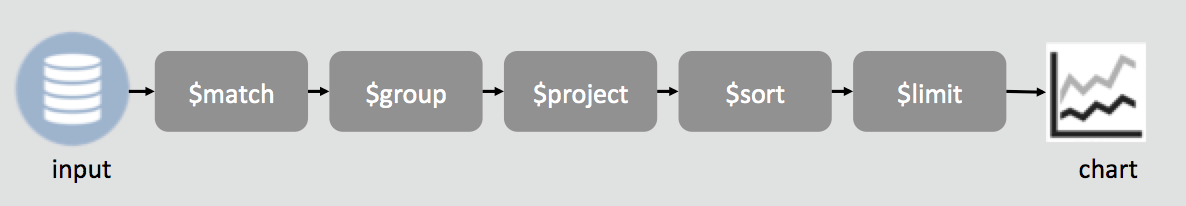 Mongo DB is a framework that allows doing manipulation
of the different data sources. We can :
Mongo DB is a framework that allows doing manipulation
of the different data sources. We can :
- Filter the data
- Do some calculations between columns (sum, subtract, multiply, divide)
- Group the data on different axis
- Sort them
- Limit the number of lines we want to keep Feel free to refer to mongo db documentation online: https://docs.mongodb.com/manual/reference/operator/aggregation-pipeline/
The steps can be used in the order you want.
To use MongoDB agregation framework, query is not an object but an
array. Here is an example of a complex MongoDB query:
chartOptions:
  data:
    query:[
      $match:
        domain: 'sugarcane_toi'
        Core: 1
        Plant: {$ne: 'BU'}
    ,
      $sort: { 'Date': -1}
    ,
      $group:
        _id: { KPI_short:'$KPI_short', Plant: '$Plant', DayType:'$DayType'}
        Actual: {$first: '$Actual'}
        Plan: {$first: '$Plan'}
        precision: {$first: '$precision'}
        unit: {$first: '$unit'}
    ,
      $project:
        Actual: 1
        Plan: 1
        unit: 1
        precision: 1
        Plant: '$_id.Plant'
        KPI_short: '$_id.KPI_short'
        DayType: '$_id.DayType'
        evolution: { $subtract: ['$Plan', '$Actual'] }
    ]
Step $match
In the match step, we can filter the data thanks to the values we
want to keep or not. Many functions can help doing that filtering :
$ne, $in, $nin:, $gt and $lt.
$ne: exclude one value$nin: exclude multiple values$in: include multiple values
Example
| country | value |
|---|---|
| France | 100 |
| France | 500 |
| Allemagne | 500 |
| France | 500 |
| France | 500 |
| Allemagne | 500 |
| Maroc | 200 |
data:
  query:[
    $match:
      domain: 'my_domain'
      country: $in: ['France', 'Maroc']
  ]
| country | value |
|---|---|
| France | 100 |
| France | 500 |
| France | 500 |
| France | 500 |
| Maroc | 200 |
Example with all filtering options:
data:
  query:[
    $match:
      domain: 'my_domain'
      column_1: 'value_in_column_1'
      column_2: $ne: "value_in_column_2"
      column_3: $nin: ["value_1", "value_2"]
      column_4: $in: ["value_1", "value_2"]
  ]
Step $project
The $project step allows doing calculation on the columns, the
inclusion of fields, the suppression of fields, the addition of new
fields, and the resetting of the values of existing fields.
You can also use the operator $addFieldsinstead of $project.
This operator is equivalent to a $project step that explicitly keep all
existing fields of the dataset and adds the new fields.
Inclusion of a field
If we want to conserve a column, we have to indicate with a boolean
1 or 0.
My dataset:
| country | category | value_1 | value_2 |
|---|---|---|---|
| France | Femme | 600 | 200 |
| France | Homme | 1000 | 100 |
| Allemagne | Femme | 500 | 500 |
| Allemagne | Homme | 500 | 400 |
| Maroc | Homme | 200 | 150 |
data:
  query:[
    $match:
      domain: 'my_domain'
  ,
    $project:
      country: 1
      value_1: 1
  ]
my output is:
| country | value_1 |
|---|---|
| France | 600 |
| France | 1000 |
| Allemagne | 500 |
| Allemagne | 500 |
| Maroc | 200 |
Calculation on metrics:
$add: [ "$column_1", "$column_2"]: creates a new column with the sum :column_1+column_2$subtract: [ "$column_1", "$column_2"]: creates a new column with the difference:column_1-column_2$multiply: [ "$column_1", "$column_2"]: creates a new column with the multiplication:column_1*column_2$divide: [ "$column_1", "$column_2"]: creates a new column with the division:column_1/column_2We can use columns but also figures. For example:$divide: [ "$column_1", 100]
my dataset is:
| country | category | value_1 | value_2 |
|---|---|---|---|
| France | Femme | 600 | 200 |
| France | Homme | 1000 | 100 |
| Allemagne | Femme | 500 | 500 |
| Allemagne | Homme | 500 | 400 |
| Maroc | Homme | 200 | 150 |
data:
  query:[
    $match:
      domain: 'my_domain'
  ,
    $project:
      country: 1
      category: 1
      value_3: $subtract: ["$value_1", "$value_2"]
  ]
My output is:
| country | category | value_3 |
|---|---|---|
| France | Femme | 400 |
| France | Homme | 900 |
| Allemagne | Femme | 0 |
| Allemagne | Homme | 100 |
| Maroc | Homme | 50 |
Add new fields or reset existing fields
To set a field value directly to a numeric or boolean literal, as
opposed to setting the field to an expression that resolves to a
literal, use the $literal operator. You can also create a new field
thanks to $concat operator.
Example my dataset is:
| country | category | value_1 | value_2 |
|---|---|---|---|
| France | Femme | 600 | 200 |
| France | Homme | 1000 | 100 |
| Allemagne | Femme | 500 | 500 |
| Allemagne | Homme | 500 | 400 |
| Maroc | Homme | 200 | 150 |
data:
  query:[
    $match:
      domain: 'my_domain'
  ,
    $project:
      country: 1
      category: 1
      test: $literal: "This is a test"
      numeric: $literal: 10
      label: $concat: [ "$country", " - ", "$category"]
  ]
My output is:
| country | category | test | numeric | label |
|---|---|---|---|---|
| France | Femme | This is a test | 10 | France - Femme |
| France | Homme | This is a test | 10 | France - Homme |
| Allemagne | Femme | This is a test | 10 | Allemagne - Femme |
| Allemagne | Homme | This is a test | 10 | Allemagne - Homme |
| Maroc | Homme | This is a test | 10 | Maroc - Homme |
Step $group
The $group step allows grouping data in 1 or multiple axis. This
step always contains:
_id: the axis of the grouping- calculus of the other columns Be careful the output of the grouping
step changes the name of the indexes columns (
_id). Always use$projectstep to rename the steps.
Example my dataset is:
| country | value |
|---|---|
| France | 100 |
| France | 500 |
| Allemagne | 500 |
| France | 500 |
| France | 500 |
| Allemagne | 500 |
| Maroc | 200 |
data:
  query:[
    $match:
      domain: 'my_domain'
  ,
    $group:
      _id:
        "country": "$country"
      value: $sum: "$value"

  ]
my output is:
_id.country |
value |
|---|---|
| France | 1600 |
| Allemagne | 1000 |
| Maroc | 200 |
Example with a multiple axis
my dataset is:
| country | category | value |
|---|---|---|
| France | Femme | 100 |
| France | Homme | 500 |
| Allemagne | Femmme | 500 |
| France | Femme | 500 |
| France | Homme | 500 |
| Allemagne | Homme | 500 |
| Maroc | Homme | 200 |
data:
  query:[
    $match:
      domain: 'my_domain'
  ,
    $group:
      _id:
        "country": "$country"
        "category": "$category"
      value: $sum: "$value"

  ]
my output is:
_id.country |
_id.category |
value |
|---|---|---|
| France | Femme | 600 |
| France | Homme | 1000 |
| Allemagne | Femme | 500 |
| Allemagne | Homme | 500 |
| Maroc | Homme | 200 |
The functions we can use to calculate the metrics are :
$sum: to sum the values on the grouping axis$avg: to calculate the average values on the grouping axis$first: to keep the first value on the grouping axis$last: to keep the last value on the grouping axis$max: to keep the maximal value on the grouping axis$min: to keep the minimal value on the grouping axis
data:
  query:[
    $match:
      domain: 'my_domain'
      column_4: $in: ["value_1", "value_2"]
  ,
    $group:
      _id:
        "axis_1": "$axis_1"
        "axis_2": "$axis_2"

      value: $sum: "$value"

  ]
Step $sort
The $sort operator sorts your input dataset and returns in a sorted
order depending on 1 or multiple fields: (numeric or alphabetic). The
order can have one of the following values:
- 1 to specify ascending order.
- -1 to specify descending order.
Example 1: sorting in an alphabetical order my dataset is:
| country | category | value_1 | value_2 |
|---|---|---|---|
| France | Femme | 600 | 200 |
| France | Homme | 1000 | 100 |
| Allemagne | Femme | 500 | 500 |
| Allemagne | Homme | 500 | 400 |
| Maroc | Homme | 200 | 150 |
data:
  query:[
    $match:
      domain: 'my_domain'
  ,
    $sort:
      "country": 1
  ]
my output is:
| country | category | value_1 | value_2 |
|---|---|---|---|
| Allemagne | Femme | 500 | 500 |
| Allemagne | Homme | 500 | 400 |
| France | Femme | 600 | 200 |
| France | Homme | 1000 | 100 |
| Maroc | Homme | 200 | 150 |
Example 2: sorting in an decreasing order my dataset is:
| country | category | value_1 | value_2 |
|---|---|---|---|
| France | Femme | 600 | 200 |
| France | Homme | 1000 | 100 |
| Allemagne | Femme | 500 | 500 |
| Allemagne | Homme | 500 | 400 |
| Maroc | Homme | 200 | 150 |
data:
  query:[
    $match:
      domain: 'my_domain'
  ,
    $sort:
      "value_1": -1
  ]
my output is:
| country | category | value_1 | value_2 |
|---|---|---|---|
| France | Homme | 1000 | 100 |
| France | Femme | 600 | 200 |
| Allemagne | Femme | 500 | 500 |
| Allemagne | Homme | 500 | 400 |
| Maroc | Homme | 200 | 150 |
Step $limit
The $limit operator limits the number of lines of your dataset.
Example my dataset is:
| country | category | value_1 | value_2 |
|---|---|---|---|
| France | Femme | 600 | 200 |
| France | Homme | 1000 | 100 |
| Allemagne | Femme | 500 | 500 |
| Allemagne | Homme | 500 | 400 |
| Maroc | Homme | 200 | 150 |
data:
  query:[
    $match:
      domain: 'my_domain'
  ,
    $limit: 2
  ]
my output is:
| country | category | value_1 | value_2 |
|---|---|---|---|
| France | Femme | 600 | 200 |
| France | Homme | 1000 | 100 |
Step $skip
The $skip operator skips the N first lines of your dataset.
Example my dataset is:
| country | category | value_1 | value_2 |
|---|---|---|---|
| France | Femme | 600 | 200 |
| France | Homme | 1000 | 100 |
| Allemagne | Femme | 500 | 500 |
| Allemagne | Homme | 500 | 400 |
| Maroc | Homme | 200 | 150 |
data:
  query:[
    $match:
      domain: 'my_domain'
  ,
    $skip: 2
  ]
my output is:
| country | category | value_1 | value_2 |
|---|---|---|---|
| Allemagne | Femme | 500 | 500 |
| Allemagne | Homme | 500 | 400 |
| Maroc | Homme | 200 | 150 |
Multiple queries
We can concat multiples mongoDB queries thanks to multiple_queries
option.
Example
domain: “France”
| category | value | value_n_1 |
|---|---|---|
| Femme | 600 | 200 |
| Homme | 1000 | 100 |
domain: “uk”
| category | value | value_last_year |
|---|---|---|
| Femme | 500 | 600 |
| Homme | 1100 | 500 |
| Unknown | 100 | 100 |
data:
  query:[
    [
      $match:
        domain: 'france'
    ,
      $addFields:
        country: $literal: "France"
    ]
    [
      $match:
        domain: 'UK'
    ,
      $project:
        category: 1
        value: 1
        value_n_1: "$value_last_year"
        country: $literal: "UK"
    ]
  ]
  multiple_queries: true
| country | category | value | value_n_1 |
|---|---|---|---|
| France | Femme | 600 | 200 |
| France | Homme | 1000 | 100 |
| UK | Femme | 500 | 600 |
| UK | Homme | 1100 | 500 |
| UK | Unknown | 100 | 100 |